Learn how to integrate CEIC data into R to access and analyze a wide range of economic indicators. Understanding how to retrieve and work with CEIC data is valuable for economic analysis.
Prerequisites
Install and Load Packages
To get started, you’ll need to install the CEIC package from the CEIC repository and load the necessary libraries.
# Install the 'ceic' package from the specified repository. install.packages("ceic", repos ="https://downloads.ceicdata.com/R/", type ="source")
# Load the necessary librarieslibrary(zoo)
Attaching package: 'zoo'
The following objects are masked from 'package:base':

    as.Date, as.Date.numeric
library(xts)library(ceic)
Environment set to: PROD
[1] "Previous session closed."
Using base url: https://api.ceicdata.com/v2
Authentication
You must log in to access the CEIC database. The ceic.login() function initiates the login process. Replace the email below with your CEIC account email and password.
If you encounter an “error in file”, you might need to manually create a folder for storing CEIC data. You can do this using the command below, and then running the login command again.
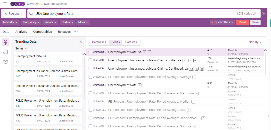
The CEIC website offers an easy user-friendly interface to allow you to explore series codes. First, login at https://www.ceicdata.com/en.
Then, browse and search by key words in the top search bar. For example, let’s look for U.S. unemployment rate. You will see multiple options pop up as available series.
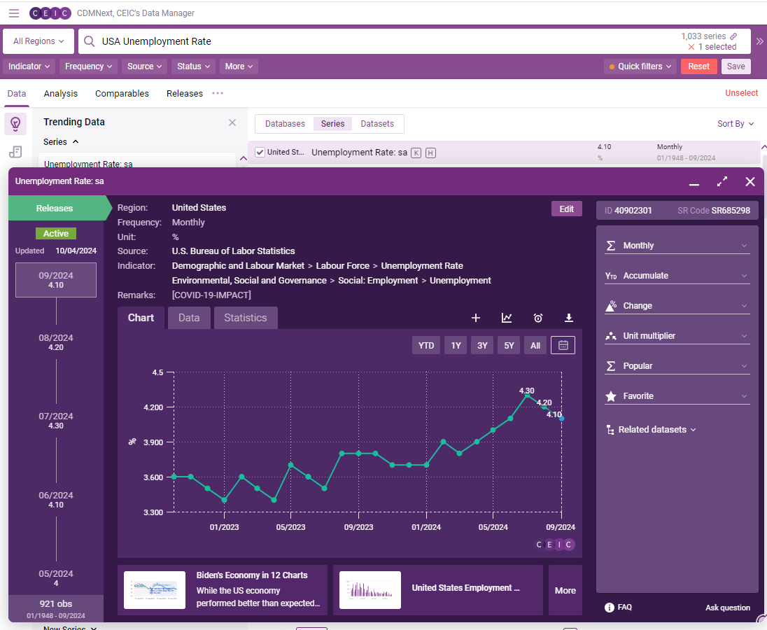
In this example, the first series that pops up is the series we are looking for. When clicking on the series, it opens a more detailed menu that allows you to see the ID, the SR Code, and some chart, data, and statistics. This is helpful if only looking for one series.
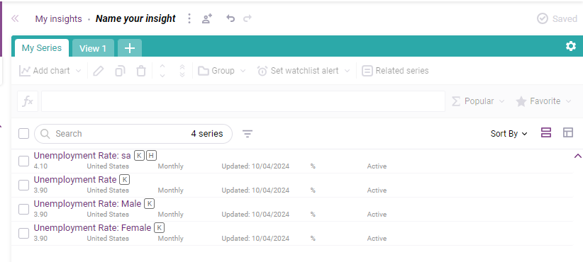
If you are looking for multiple series, you can drag them into the my insights panel. Let’s use for example four different unemployment series for the U.S. Your insights panel should look something like this.
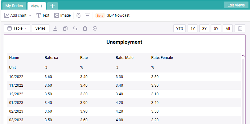
If you click on the default view, ‘View 1’, you can easily visualize the data as a graph or a table. You will also notice a button on the top left called ‘series’.
When clicking on the ‘Series’ button in your view, it allows you to see the key information for your series, and most importantly the series IDs.
Retrieving the series code in R
Now that we have easily identified the series codes we are looking for, we can retrieve them in R using their ID. Let’s first start by retrieving the general seasonally adjusted unemployment series for the U.S.
# Retrieve time series using its IDsa_unemp_us <-ceic.series(40902301)
We can optionally view the structure of the series, giving a more detailed view of the timepoints and metadata using the command ‘View’.
View(sa_unemp_us)
The retrieved data is structured as a list with two key components:
Metadata: Contains information like the name, frequency, unit, and source of the data.
Timepoints: Stores the actual time series data.
We can also quickly plot the data to visualize what it looks like using this command.
#Plot all available dataplot(sa_unemp_us$timepoints,main=sa_unemp_us$metadata$name)
Downloading Multiple Time Series
If we want to download all the other unemployment series codes we were looking at, we would do it by defining a vector of series IDs, and then retrieving them. Here, we retrieve the timepoints and metadata separately.
# Define a vector of series IDsunempl_ids <-c('40952001', '40953401', '40954701')# Retrieve data for all seriesmulti_unempl_data <-ceic.timepoints(unempl_ids)# Retrieve metadata for all seriesmulti_unempl_metadata <-ceic.metadata(unempl_ids)
Merging and Structuring the Data
Once we have retrieved multiple time series data from CEIC (in this case, multiple U.S. unemployment-related series), we often want to combine them into a single dataset for comparison or further analysis. This is particularly useful if you want to compare trends across different variables over the same time period.
When you retrieve multiple time series from CEIC, they are stored as individual objects within a list. To work with these multiple series as a single dataset, we need to merge them. The do.call("merge", ...) function in R is a convenient way to combine the individual zoo time series into a single object.
The do.call() function applies a function (in this case, merge) to all elements in a list.
merge() aligns the time series based on their dates. If there are missing values for any series on a particular date, the result will include NA for those points.
Here is the code that merges the unemployment time series data, also giving you a preview of the new aligned series at the end.
# Merge the time series data merged_data <-do.call("merge", multi_unempl_data) # Set column names based on series names from metadata colnames(merged_data) <- multi_unempl_metadata$name #View the tail end of the datatail(merged_data)
           Unemployment Rate Unemployment Rate: Male Unemployment Rate: Female
2025-08-01               4.5                     4.3                       4.8
2025-09-01               4.3                     4.2                       4.4
2025-10-01                NA                      NA                        NA
2025-11-01               4.3                     4.4                       4.3
2025-12-01               4.1                     4.2                       3.9
2026-01-01               4.6                     4.9                       4.4
The merging process ensures three main things:
Time Alignment: time series are aligned along the same timeline. For example, if one series has data starting in 2000, and another starts in 2005, the merged dataset will have NA values for the earlier years for the second series, ensuring consistency in the time index.
Column Naming: After merging, each column in the resulting dataset corresponds to one of the time series. The column names are derived from the metadata of the series, allowing you to easily identify which series each column represents.
Handling Missing Data: If one or more series have missing data for a certain time period, the merged dataset will include NA in those places.
Now, you have a single time series object containing multiple variables which can be used for further analysis.
Visualizing the Merged Data
You can easily visualize the merged dataset by plotting the series together, comparing their trends over time. For example, let’s visualize the three time series we have retrieved all in separate plots side by side for the time period of 2000 to the most recently available data.
# Define the range of interest as Date objectsstart_date <-as.Date("2000-01-01")end_date <-Sys.Date()# Subset the merged data based on the date rangesubset_data <- merged_data[index(merged_data) >= start_date &index(merged_data) <= end_date]# Set up the plotting area to have 3 rows and 1 column (stacked plots)par(mfrow =c(3, 1))# Plot each series separately, stacking them verticallyplot.zoo(subset_data[, 1], main =colnames(subset_data)[1], xlab ="Date", ylab ="Value", col ="blue")plot.zoo(subset_data[, 2], main =colnames(subset_data)[2], xlab ="Date", ylab ="Value", col ="green")plot.zoo(subset_data[, 3], main =colnames(subset_data)[3], xlab ="Date", ylab ="Value", col ="red")
This provides a simple way to combine CEIC’s powerful dataset retrieval, with R’s flexible time series handling to easily manipulate, merge and visualize economic data.
Data Exploration Directly in R
We first explored how to search for data using the CEIC website. Now, we will explore how to find data from CEIC directly in R.
Exploring Classifications
Classifications group data into meaningful categories, such as regions, sectors, or types of economic indicators. This structure allows for efficient filtering and searching through CEIC’s large datasets. For example, classifications may help you locate all datasets related to balance of payments, banking statistics, interest rates and more.
We can explore available classifications in CEIC directly in R using the following command:
                                    name     id
1                      National Accounts 200016
2                             Production 200017
3  Sales, Orders, Inventory and Shipment 200018
4                           Construction 200019
5             Properties and Real Estate 200020
6          Government and Public Finance 200021
7                            Demographic 200022
8                          Labour Market 200023
9    Domestic Trade and Household Survey 200024
10                         Foreign Trade 200025
11                    Balance of Payment 200026
12                   Inflation and Price 200027
13                              Monetary 200028
14                    Banking Statistics 200029
15                      Foreign Exchange 200030
16                         Interest Rate 200031
17                            Investment 200032
18                       Commodity Price 200033
19          Business and Economic Survey 200034
20                               Tourism 200035
21                             Transport 200036
22      Technology and telecommunication 200037
23                      Financial Market 200038
By understanding the classifications, you can focus on relevant data categories improving the efficiency of your analysis.
Searching for Data Series in R
CEIC offers many datasets, and you can search for specific data series using keywords, regions, and other filters. Here, we will search for the “Industrial Production Index” in G7 countries, focusing only on monthly data.
# Search for the Industrial Production Index in G7 countriessearch_result <-ceic.search(keyword ="Industrial Production Index", #add the keywordregion =ceic.regions("G7"), #add the regionsubscribed_only =TRUE, frequency ="M", #add the frequencysource =ceic.sources("CEIC Data") #looks at the entire CEIC data)
# Display the top search resultshead(search_result)
         id                                                         name unit
1 211484702 Industrial Production Index: YoY: Monthly: sa: United States    %
2 249416501         Industrial Production Index: YoY: Monthly: sa: Japan    %
3 414412097            Industrial Production Index: YoY: Monthly: Canada    %
4 211824902     Industrial Production Index: YoY: Monthly: swda: Germany    %
5 211190702      Industrial Production Index: YoY: Monthly: swda: France    %
6 292860502        Industrial Production Index: YoY: Monthly: sa: Canada    %
        country province frequency status    source  startDate    endDate
1 United States     <NA>   Monthly Active CEIC Data 1920-01-01 2026-01-01
2         Japan     <NA>   Monthly Active CEIC Data 1954-01-01 2026-01-01
3        Canada     <NA>   Monthly Active CEIC Data 1958-01-01 2023-10-01
4       Germany     <NA>   Monthly Active CEIC Data 1959-01-01 2025-12-01
5        France     <NA>   Monthly Active CEIC Data 1991-01-01 2025-12-01
6        Canada     <NA>   Monthly Active CEIC Data 1958-01-01 2026-01-01
  multiplierCode            lastUpdateTime  timepointsLastUpdateTime keySeries
1             NA 2026-02-18T14:33:13+00:00 2026-02-18T14:31:48+00:00     false
2             NA 2026-02-27T00:12:16+00:00 2026-02-27T00:04:26+00:00     false
3             NA 2024-04-18T11:58:03+00:00 2024-03-06T10:40:25+00:00     false
4             NA 2026-02-06T07:48:30+00:00 2026-02-06T07:48:08+00:00     false
5             NA 2026-02-05T08:48:43+00:00 2026-02-05T08:44:04+00:00     false
6             NA 2026-02-27T14:00:13+00:00 2026-02-27T13:58:03+00:00     false
  periodEnd classification indicator remarks replacements           mnemonic
1        31           <NA>      <NA>                 <NA> US.IPI.VO.SA-YoY-M
2        31           <NA>      <NA>                 <NA> JP.IPI.VO.SA-YoY-M
3        31           <NA>      <NA>                 <NA>
4        31           <NA>      <NA>                 <NA> DE.IPI.VO.SA-YoY-M
5        31           <NA>      <NA>                 <NA> FR.IPI.VO.SA-YoY-M
6        31           <NA>      <NA>                 <NA> CA.IPI.VO.SA-YoY-M
  isForecast hasVintage isHeadline  hasContinuousSeries hasSchedule seriesTag
1      false      false       false               false       false  UBHAAAAAA
2      false      false       false               false       false JBAAAAAAAA
3      false      false       false               false       false
4      false      false       false               false       false EBAAAAAAAA
5      false      false       false               false       false  FRBABAAAA
6      false      false       false               false       false
  subscribed
1       true
2       true
3       true
4       true
5       true
6       true
Looking at the top portion of the search result might not provide a clear enough picture of the data structure you are looking at. Let’s dive into the details.
Data Structure
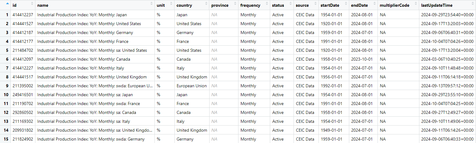
When you retrieve data from CEIC using ceic.search(), the result is structured as a data frame. Each row represents a data series, and columns provide metadata, including the name, region, frequency, source, and unique ID for that series. If we use the View function, we can optionally view the entire data frame in a new window. For example:
# Optionally view the data frameView(search_result)
You’ll see a table with columns like:
ID: The unique identifier for each series.
Name: A brief description of the series (e.g., “Industrial Production Index”).
Country: The geographical area to which the data applies (e.g., “United States”).
Frequency: The data frequency (e.g., “Monthly”).
Start Date: The date which the data series starts.
End Date: The date which the data series ends.
Last updated time: The date which the series was last updated.
This structure helps you understand what kind of data you’re working with and provides critical metadata for further analysis.
You can retrieve data in R in the same way we explored earlier, using the series codes directly. This approach lets you explore data directly in R instead of using the website interface.
You’ve learned how to access, explore, and retrieve data from CEIC.
 You’ll see a table with columns like: