IMF Datatools

Learn how to install IMF Datatools and access data in R. IMF Datatools is a Python library that provides access to various internal and external data sources, which you can use directly in R.

Pre-requisites

Since IMF Datatools is Python based, we first need download Python 3.11 or above from the IMF Software Center and install our Python library.

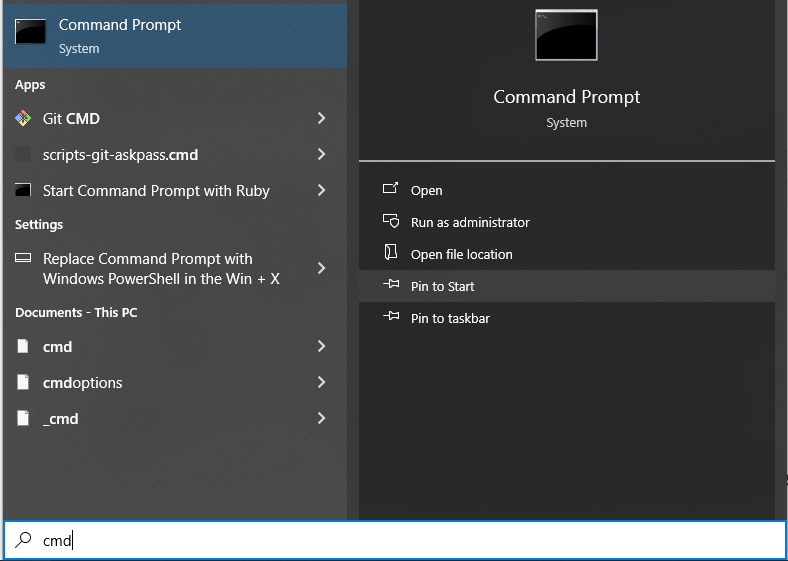
After you have downloaded Python 3.11 or the latest version from the IMF Software Center, open the Command Prompt. You can load this by typing “cmd” in the Windows search option, as shown below.

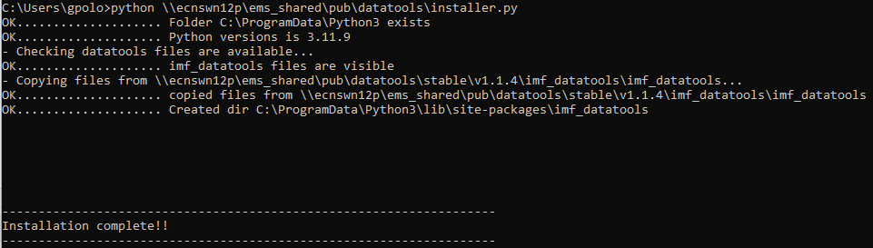
In the command prompt, type the following command to install Datatools.

python \\ecnswn12p\ems_shared\pub\datatools\installer.py dev

You should generate something similar to the following message when the installation is complete.

Loading the Python Interpreter

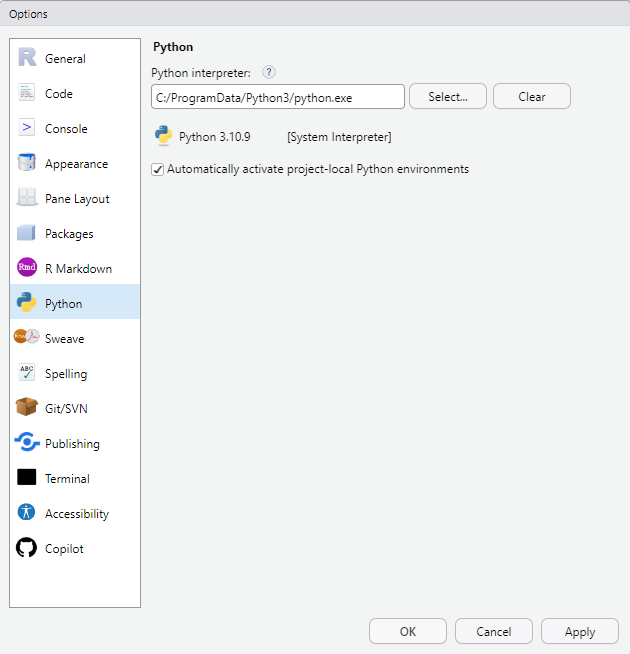
After Python 3.11 is downloaded and Datatools is installed, we need to load it into R Studio. To use IMF Datatools in RStudio, you need to set the location of your Python interpreter.

In the menu tab of R Studio, go to Tools, Global Options, choose Python and then select the interpreter from your computer. When you click select, it should automatically populate under system after download. Click Apply and OK.

Your R session will likely need to be restarted to ensure the changes take into effect. This process only needs to be done once.

Loading additional packages

To bridge the communication between R and Python, you will also need to install and load the reticulate package, only once.

#install.packages("reticulate")
library(reticulate)

Handling Dates in Reticulate

When using the reticulate package to work with IMF Datatools, it is important to note that reticulate interprets dates in UTC time by default. This can lead to incorrect date stamps when downloading data if your system time is set to a different timezone.

To prevent this issue, you must set your system timezone to UTC before retrieving data. You can do this in R by running:

Sys.setenv(TZ = "UTC")

Lastly, you will need to import the sys module and the IMF Datatools library for calling from R.

sys <- import("sys")
imf_datatools  <-  import("imf_datatools")

You should now be set up to use IMF Datatools in R Studio.

Further documentation on IMF Datatools can also be found at this link.

Datasets available in IMF Datatools

Understanding the available data

IMF Datatools has direct access to a plethora of internal and external databases like Haver, OECD, and more. For exploratory work, you can view all the databases or import a specific database.

Utilizing the function imf_datatools$ in your console, you are interacting with an object which allows you to navigate available Datatools utilities using the $ operator. This will trigger an auto-complete pop-up showing the available modules (e.g., external data utilities, internal tools, metadata helpers).

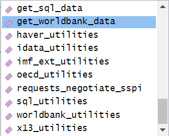
With this information, you can then import a specific library under IMF Datatools, e.g., OECD. These “libraries” act as connectors that contain multiple functions for accessing data, metadata, and reference tables.

#Import a specific library under IMF Datatools, e.g., EDI 
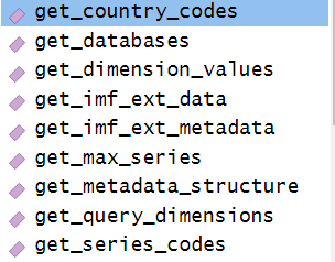
imf_ext_utilities <- imf_datatools$imf_ext_utilities

Within that library, you can then explore the functions within to get data, country codes, metadata, and more. Each utility typically includes functions to list available datasets, retrieve series, map country identifiers, and inspect metadata. You would explore this functionality by also utilizing the $ sign.

#You can then look at the functionality 
imf_ext_utilities$

At this stage, you can explore functions that:

• List available datasets or series

• Retrieve time series data

• Return country or entity code mappings

• Expose metadata and documentation

After exploring the available connectors, we can now use them to pull actual datasets into our R session for analysis.

Using the datasets available in IMF Datatools

Let’s now download some series directly from these databases.

Using Haver data

For Haver data, make sure to specify the series and the database, such as GDP@USECON.

#Download Haver series for one country 
df  <-  imf_datatools$get_haver_data('GDP@USECON')

#Quickly glance at the tail end of the data
tail(df)

           GDP@USECON
2024-07-01    29511.7
2024-10-01    29825.2
2025-01-01    30042.1
2025-04-01    30485.7
2025-07-01    31098.0
2025-10-01    31490.1

You can also download multiple series in one command, but make sure they have compatible scales.

#Download multiple series in one command
df <- imf_datatools$get_haver_data(c('PJ4@USECON', 'PCUP@USECON'))

#Quickly glance at the tail end of the data
tail(df)

           PJ4@USECON PCUP@USECON
2025-08-01       -0.2         0.3
2025-09-01        0.6         0.3
2025-10-01        0.1         NaN
2025-11-01        0.2         NaN
2025-12-01        0.4         0.3
2026-01-01        0.5         0.2

If you need more info on the scales, you can easily browse the metadata for an indicator.

#Obtain details on the metadata for a particular series
metadata <- imf_datatools$haver_utilities$get_haver_metadata('GDP@USECON')

#Quickly glance at the tail end the metadata
tail(metadata)

    database  startdate    enddate frequency
gdp   usecon 1947-03-31 2025-12-31         Q
                              descriptor numobs         datetimemod magnitude
gdp Gross Domestic Product (SAAR, Bil.$)    316 2026-02-20 13:32:00         9
    decprecision diftype aggtype datatype group geography1 geography2
gdp            1       0     AVG      US$   N01        111           
    shortsource                  longsource
gdp         BEA Bureau of Economic Analysis

Using World Bank data

You can also access World Bank data, but make sure you denote country abbreviation instead of IMF country code.

# Download series for population in USA from World Bank DAta
df  <-  imf_datatools$get_worldbank_data('SP.POP.TOTL', 'USA')

#Quickly glance at the tail end of the data
tail(df)

           USA.SP.POP.TOTL
2020-01-01       331577720
2021-01-01       332099760
2022-01-01       334017321
2023-01-01       336806231
2024-01-01       340110988
2025-01-01             NaN

Using Bloomberg data

Bloomberg data typically accessible via iData can also be accessed, ensuring the correct nomenclature.

#Download daily Vix Index Bloomberg data
df  <-  imf_datatools$get_ecos_bloomberg_data('VIX Index', 'PX_LAST')

#Quickly glance at the tail end of the data
tail(df)

           VIX IndexPX_LAST.D
2026-02-26              18.63
2026-02-27              19.86
2026-02-28                NaN
2026-03-01                NaN
2026-03-02              21.44
2026-03-03              23.57

Now you’ve got IMF Datatools installed, understood the available datasets, and downloaded relevant series.

Using iData

The new Fund‐wide iData (2025) replaces EcOS, EDI, and can be accessed via the reticulate package. This is slightly different than the other sites as it includes both publicly available and private datasets. Let’s explore those below.

In order to access publicly available datasets, you need to specify that no token is needed via stating “FALSE” below. Let’s explore how to see the public datasets in iData below.

#alias the imported Python module for brevity of calls
dt <- imf_datatools

#Public datasets (no token needed)
dt$idata_utilities$PRIVATE <- FALSE
head(dt$idata_utilities$get_databases())

                                                                           name
IMF.STA:NSDP                                  National Summary Data Page (NSDP)
IMF.STA:MFS_DC Monetary and Financial Statistics (MFS), Depository Corporations
IMF.STA:PI_WCA           Production Indexes, World and Country Group Aggregates
IMF.STA:FAS                                       Financial Access Survey (FAS)
IMF.STA:FD                                         Fiscal Decentralization (FD)
IMF.STA:ER                                                  Exchange Rates (ER)
               Agency ID Resource ID Latest Version             Unique ID
IMF.STA:NSDP     IMF.STA        NSDP          7.0.0   IMF.STA:NSDP(7.0.0)
IMF.STA:MFS_DC   IMF.STA      MFS_DC          8.0.0 IMF.STA:MFS_DC(8.0.0)
IMF.STA:PI_WCA   IMF.STA      PI_WCA          1.0.0 IMF.STA:PI_WCA(1.0.0)
IMF.STA:FAS      IMF.STA         FAS          4.0.0    IMF.STA:FAS(4.0.0)
IMF.STA:FD       IMF.STA          FD          6.0.0     IMF.STA:FD(6.0.0)
IMF.STA:ER       IMF.STA          ER          4.0.1     IMF.STA:ER(4.0.1)

You can also list your private datasets, which you have access to.

#Private datasets based on your access level
dt$idata_utilities$PRIVATE <- TRUE
head(dt$idata_utilities$get_databases())

                                                                           name
IMF.STA:NSDP                                  National Summary Data Page (NSDP)
IMF.STA:MFS_DC Monetary and Financial Statistics (MFS), Depository Corporations
IMF.STA:PI_WCA           Production Indexes, World and Country Group Aggregates
IMF.STA:FAS                                       Financial Access Survey (FAS)
IMF.STA:FD                                         Fiscal Decentralization (FD)
IMF.STA:ER                                                  Exchange Rates (ER)
               Agency ID Resource ID Latest Version             Unique ID
IMF.STA:NSDP     IMF.STA        NSDP          7.0.0   IMF.STA:NSDP(7.0.0)
IMF.STA:MFS_DC   IMF.STA      MFS_DC          8.0.0 IMF.STA:MFS_DC(8.0.0)
IMF.STA:PI_WCA   IMF.STA      PI_WCA          1.0.0 IMF.STA:PI_WCA(1.0.0)
IMF.STA:FAS      IMF.STA         FAS          4.0.0    IMF.STA:FAS(4.0.0)
IMF.STA:FD       IMF.STA          FD          6.0.0     IMF.STA:FD(6.0.0)
IMF.STA:ER       IMF.STA          ER          4.0.1     IMF.STA:ER(4.0.1)

Once you’ve picked a database (e.g. "IMF.STA:CPI"), you can also check its structure.

• get_dimensions() lists all the ways you can slice your data, i.e., by country, frequency etc.

dims <- dt$idata_utilities$get_dimensions("IMF.STA:CPI")
print(dims)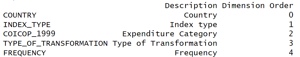

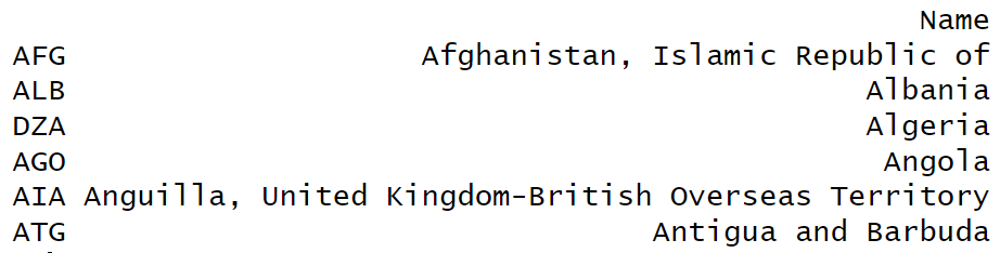
• get_dimension_values() this function provides the full list of entries within a specific dimension, e.g., Country.

  vals <- dt$idata_utilities$get_dimension_values("IMF.STA:CPI", "COUNTRY")
  head(vals)

Retrieving a series

Once you have itentified your dataset and explored its dimensions you can build a query by joining dimension codes with period. Leave the key specifications empty to include all values as shown below.

# Example: CPI level for USA & JPN monthly (_T = level, M = monthly)
key <- "USA+JPN.CPI._T..M"
df  <- dt$idata_utilities$get_idata_data("IMF.STA:CPI", key)
tail(df)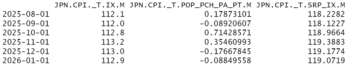

• To obtain data in long format, add longformat = TRUE.

  # Long
  key <- "USA+JPN.CPI._T..M"
  lf <- dt$idata_utilities$get_idata_data("IMF.STA:CPI", key, longformat = TRUE)
  tail(lf)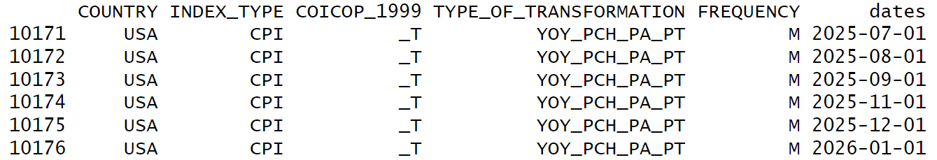

  

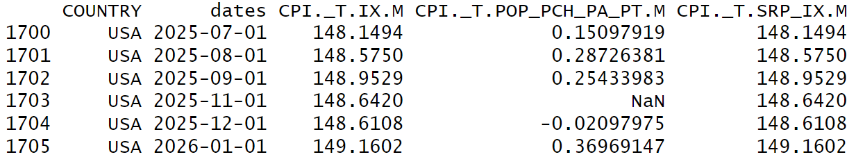
• To pivot by a dimension (e.g. COUNTRY), use panel = "COUNTRY"

  # Panel by country
  pf <- dt$idata_utilities$get_idata_data("IMF.STA:CPI", key, panel = "COUNTRY")
  tail(pf)

IMF Datatools makes it easy to browse, inspect, and retrieve IMF datasets in R.